


Plan Smarter in Simple Steps
Supporting planners to save time
How It Works
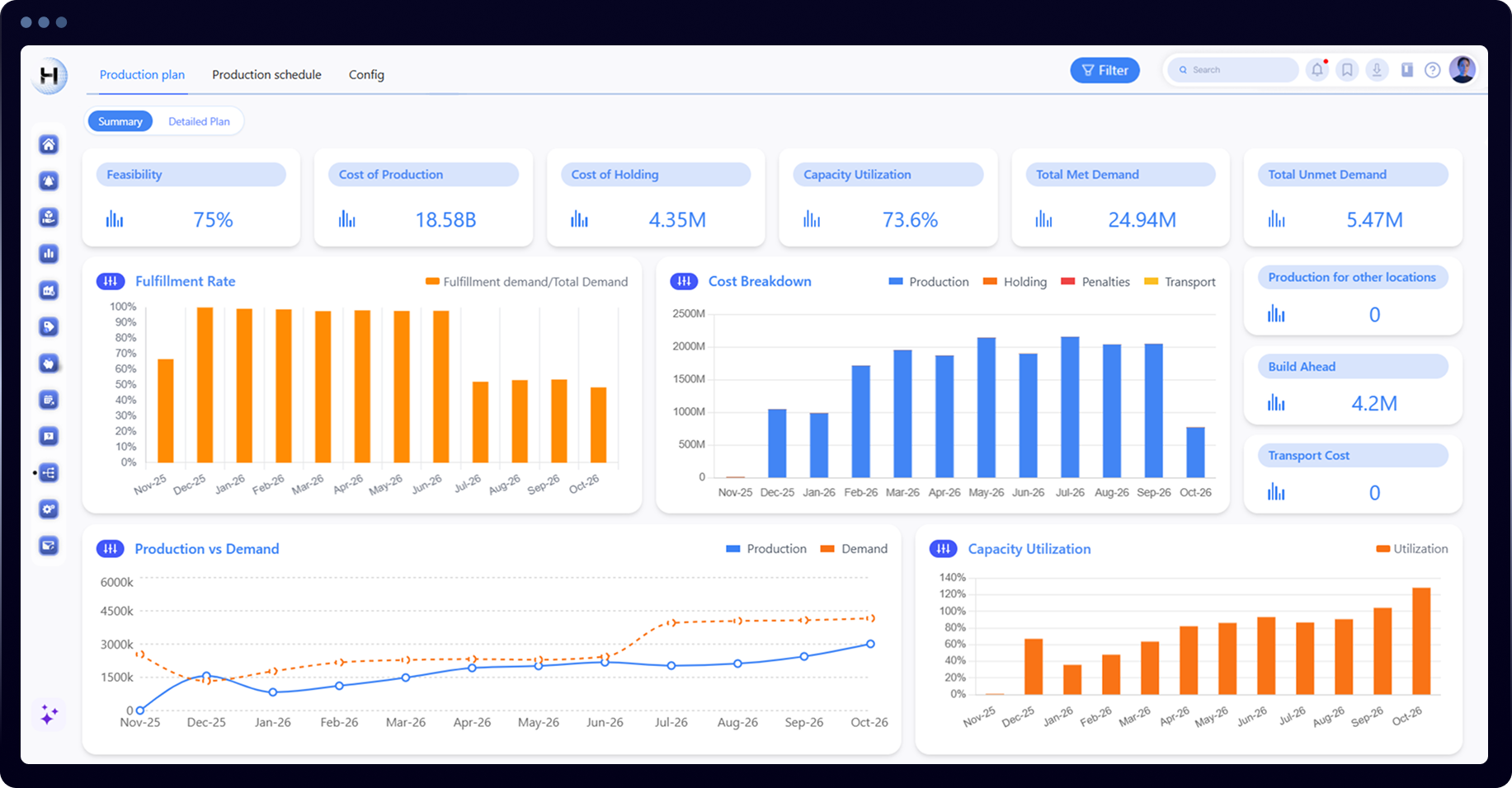
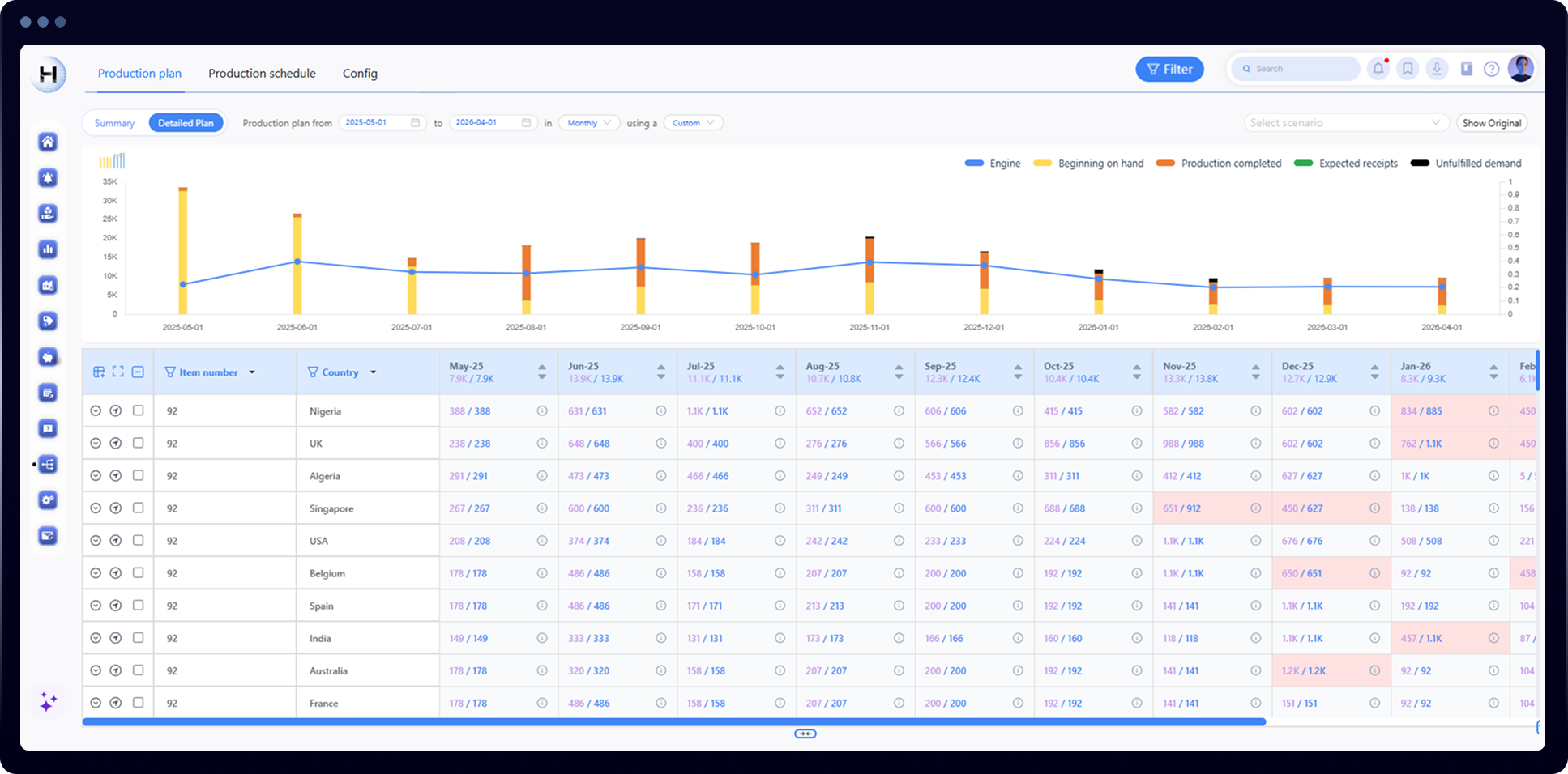
Production and Capacity Planning
Compare scenarios to maximize throughput.
.svg)
Real-time optimizer

Create feasible production plans that respect capacity, shifts, and priorities automatically.

Rough-cut capacity planning
Get instant visibility of planned versus available capacity with bottleneck detection.
.svg)
Scenario simulation
Test alternative production strategies and choose the plan with best utilization.
.svg)
Constraint management
Adjust production limits, lead times, or batch sizes and recalculate in seconds.
.svg)
Automated planning proposals
Receive optimized production suggestions with clear logic and full transparency.
.svg)
Integrated planning view
Stay aligned with demand, inventory, and scheduling.
Next-Gen Planning
Supporting planners to save time
Everything in one place.


Planners' Voices
What planning leaders say
Real experiences from planners and leaders.
"Impressed by the knowledge and fast results of Horizon.
Together we turned plans into action in no time."
Together we turned plans into action in no time."

Olivier Van Hoef –
Supply chain manager at Ahrend
Supply chain manager at Ahrend
"After 40+ years of implementing different planning tools, Horizon is by far the easiest to set up and adapt. It combines strong models with a flexibility we haven’t seen elsewhere."

Alex Young –
Director at Demand Integration
Director at Demand Integration
“What stood out was how quickly our team could use Horizon and how easily it was integrated with our current systems: the planning team saw the impact on their day-to-day immediately, and it improved collaboration and decision-making from a management perspective.”

Siddhant Bhalinge –
CEO at Ugaoo
CEO at Ugaoo
FAQ
Frequently Asked Questions
Find quick answers to the most common questions about our trading dashboard.
How do manufacturers effectively balance production and capacity to meet demand without overloading resources?
Balancing production and capacity isn’t just about numbers it’s about aligning people, machines, and materials to run efficiently without burning out resources.
In simple terms, production and capacity planning decides what to make, when to make it, and how much to make typically at a weekly or monthly level.
The key is to match production schedules with available capacity while managing real-world constraints such as:
Workforce shifts and availability
Machine cleaning, maintenance, and downtime
Energy costs and working hours
Holiday schedules and demand peaks Done right, this planning avoids last-minute rushes, idle capacity, and excess inventory.
It gives planners visibility to decide whether to advance production, maintain safety stock, or delay runs, helping businesses stay agile, cost-efficient, and ready for customer demand.
How are AI and Machine Learning transforming production planning in modern factories?
AI isn’t replacing planners it’s making them more powerful.
While machine learning excels at forecasting demand and predicting trends, the actual production planning still relies heavily on optimization models like Linear Programming (LP) and Mixed Integer Programming (MIP).
That said, AI adds tremendous value by:
Translating constraints: Turning complex business rules into parameters planners can work with.
Predicting disruptions: Identifying bottlenecks or delays before they happen.
Supporting decisions: Learning from past data to recommend efficient machine and labor utilization.
In short, AI makes planning smarter and more proactive, but the heart of production scheduling still beats through solid optimization science.
What are common challenges in capacity planning?
Supply chains often struggle with fluctuating demand, unpredictable supplier performance, and limited visibility across teams. Other challenges include inaccurate forecasts, siloed planning processes, and slow responsiveness to market changes. Without a connected planning system, capacity decisions become reactive instead of strategic.
How does production planning software improve efficiency compared to manual scheduling?
Manual scheduling worked when operations were simple. But as product lines expand and supply chains grow complex, spreadsheets can’t keep up.
That’s where production planning software steps in.
It helps planners move from reactive firefighting to proactive optimization.
Here’s how:
Automated constraint-based scheduling: Handles thousands of variables like cost, capacity, and deadlines.
Capacity balancing: Distributes workload evenly across plants or shifts.
Scenario simulation: Lets you test “what-if” scenarios before making decisions.
Optimization over guesswork: Evaluates millions of possible schedules to find the best one.
With software-driven planning, you get data-backed decisions, faster schedules, and fewer last-minute surprises—a true digital advantage for manufacturing teams.
How does Horizon help manufacturers plan production and capacity more intelligently?
At Horizon, we’ve built our Production and Capacity Planning module with one goal: help manufacturers turn complexity into clarity.
Here’s how Horizon empowers planning teams:
Built-in optimization models: Ready-to-use algorithms fine-tuned for manufacturing challenges.
Customizable constraints: Easily adapt plans for your labor rules, energy costs, or supplier limitations.
Priority-based scheduling: Focus on high-margin or urgent orders automatically.
Material synchronization: Align production runs with raw material availability to prevent stoppages.
With Horizon, planners don’t just create schedules they orchestrate operations that are faster, smarter, and more resilient. It’s the next step toward truly intelligent manufacturing planning."
Horizon Solutions empowers you to plan smarter, stay in control, and drive confident supply-chain decisions.


© 2026 Horizon Solutions. All rights reserved.